Using Historical Data to Simulate Truck Journey Durations & CO2 Emissions

Assume you own a truck company: your company takes transport orders from customers who want goods delivered from point A to point B. You are interested in the question "If one of my trucks drives from A to B, how long will that take, and how much CO2 will be emitted?" You are already thinking about tackling questions like "how can my transports emit less CO2" in the future.
In the past year, you recorded your trucks' travel data: GPS positions along with timestamps. You are mapping these positions to a road network that contains the roads and places that are most relevant to your business.
To answer your question, you want to model how future trucks will behave. You make the following assumptions:
Trucks of the future will behave similarily to historical trucks; i.e. traffic conditions, speed limits, driver breaks etc. of the future will be similar to the past.
You want to control how a simulated truck moves along the roads in a flexible way: for starters, you want to assume that truck drivers know how long it will take to travel along a certain road, and choose the quickest route to the goal, but you want to try other things in the future (e.g. allowing trucks to be loaded onto a cargo train).
This blog post will walk you through building a Python application that implements a simple model that can serve as a starting point for further exploring your question.
We will quote relevant parts of the source code right away; the full code can be found here for your viewing & executing pleasure.
Designing the simulator
Let's start with a simplified road network derived from the real world.
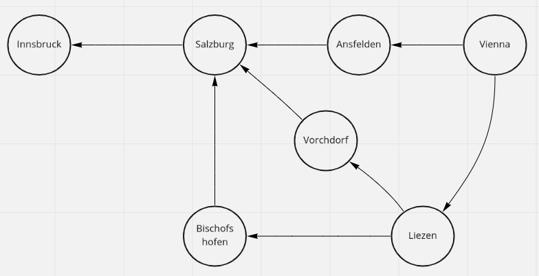
Road Network
Your most important transports take place from Vienna to Salzburg, and you determined from your tracking data that your trucks often pass close to the towns of Liezen, Ansfelden etc. You also determined that your trucks move from Liezen to Vorchdorf, but never from Bischofshofen to Vorchdorf. These observations went into building this simplified network for the simulator.
Let's call each point on the map a Location, and each edge between two points a Road:
class Location:
    def __init__(self, name: str):
        self.name = name

class Road:
    def __init__(self, start: Location, end: Location):
        self.start = start
        self.end = end

class Map:
    def __init__(self, locations: List[Location], roads: List[Road]):
        self.locations = locations
        self.roads = roads
To simulate traveling through the map, we need some information about roads. We want to start out simple, but be able to add more information later to improve our simulation:
class MovementModel:
    def get_duration_minutes(self, r: Road) -> float:
        pass

    def get_co2_kg(self, r: Road) -> float:
        pass
When simulating traveling through the map, we also need to make, at each point, a decision where to go next. The abstract decision-making process will be formalized in the simulator core: we assume that the decision will be based on the goal to minimize some metric, e.g. the travel time or the CO2 emissions. To be able to change the metric without changing the simulator core, we introduce
class DecisionMetric:
   def get_metric(self, r: Road, m: MovementModel) -> float:
      pass
To be more precise, we will assume that we want to minimize a metric for the whole route, and that the metric of the whole route is the sum of the metrics of the the roads that have been taken. This is a sensible assumption: it holds for the travel time as well as the CO2 emissions.
These assumptions allow our simulator to be based on Dijkstra's algorithm.
We end up with the following signature for our simulation method:
def simulate(map: Map, start: Location, end: Location, movement_model: MovementModel, decision_metric: DecisionMetric) -> Route:
  pass
where Route consists of the list of roads that make up the route taken by the simulator:
class Route:
  def __init__(self, legs: List[Road]):
    self.legs = legs
Implementing the simulator core
As indicated in the last section, we already made some design decision based on the idea that we will use Dijkstra's algorithm as the core of the simulator. Thus the implementation of simulate looks like this
def simulate(map: Map, start: Location, end: Location, movement_model: MovementModel, decision_metric: DecisionMetric) -> RouteResult:
    queue = PriorityQueue()
    queue.put((0, _Trip(start, None)))

    visited = []

    while not queue.empty():
        (clock, trip) = queue.get()

        if trip.location in visited:
            continue

        if trip.location == end:
            return RouteResult(Route(trip.to_list()), movement_model)

        visited.append(trip.location)

        roads = [ (road.end, road) for road in map.roads if road.start == trip.location ]

        for destination, road in roads:
            if destination in visited:
                continue

            metric = decision_metric.get_metric(road, movement_model)
            total_metric = clock + metric
            next_hop = _Trip(destination, trip)
            queue.put((total_metric, next_hop))
If you don't know Dijkstra's algorithm, feel free to continue reading without understanding all the details in the algorithm above. If you do, note that PriorityQueue from the queue module is an elegant way to implement the choice of which location to "visit" next. Remember that the while loop invariant in Dijkstra's algorithm is "we know the fastest route to each location in visisted" - thus we can finish the simulation instead of putting end into visited.
Remember: the algorithm always returns the "fastest route" from start to end. In our design, the notion of "fastest route" actually means "route with minimal metric" - what that is exactly is controlled via the decision_metric.
The following metric will cause the simulator to find a route that takes the least amount of time:
class DurationDecisionMetric:
   def get_metric(self, r: Road, m: MovementModel) -> float:
      return m.get_duration_minutes(r)
While this one will cause the simulator to find a route that emits the least amount of CO2:
class Co2DecisionMetric:
   def get_metric(self, r: Road, m: MovementModel) -> float:
      return m.get_co2_kg(r)
Or we can consider both duration and CO2 with a weighted sum:
class Co2AndDurationDecisionMetric:
   def get_metric(self, r: Road, m: MovementModel) -> float:
      return 0.8*m.get_co2_kg(r) + 0.2*m.get_duration_minutes(r)
The only thing missing from running the simulator are a Map - telling the simulator which locations exist, and which pairs are connected via a road - and a MovementModel.
We can get started with the Map by simply hardcoding the picture from the start of this section:
vienna = Location('Vienna')
liezen = Location('Liezen')
[...]
locations = [vienna, liezen, ...]

vienna_to_liezen = Road(vienna, liezen)
[...]
roads = [vienna_to_liezen, ....]

map = Map(locations, roads)
The MovementModel is not as straight-forward: how do we know how long it takes a truck to drive from Vienna to Liezen, and how much CO2 it emits? We will deal with this question in the next section; for now let's just assume each road takes exactly 1 minute to traverse, and 1 kg of CO2 is emitted, just so that we can try out simulate:
class ConstantMovementModel:
    def get_duration_minutes(self, r: Road) -> float:
        return 1

    def get_co2_kg(self, r: Road) -> float:
        return 1
Finally, everything is in place and we can run simulate. As we expected, our simulator determines that the fastest route is
Route: ['Vienna -> Ansfelden', 'Ansfelden -> Salzburg', 'Salzburg -> Innsbruck']
Duration: 3m
CO2 emissions: 3kg
Since we are planning to compute the map from our historical data, we can move this hardcoded setup into a unit test and move to parsing & using the historical data.
Considering historical data
Remember that in the first section of this post, we assumed that
In the past year, you recorded your trucks' travel data: GPS positions along with timestamps. You are mapping these positions to a road network that contains the roads and places that are most relevant to your business.
So we'll assume that the data is available as a CSV file that looks like this:
FROM,TO,DURATION_MINUTES,AVERAGE_SPEED_KMH
"Vienna","Liezen",275.43,76.26
"Vienna","Liezen",210.27,72.92
"Liezen","Vorchdorf",64.53,70.85
"Liezen","Vorchdorf",54.88,66.34
"Liezen","Vorchdorf",59.33,76.02
"Vienna","Ansfelden",101.20,59.10
Let's start by loading the data (using our previously defined Road class):
class RoadData:
    def __init__(self, duration_minutes: float, average_speed_kmh: float):
        self.duration_minutes = duration_minutes
        self.average_speed_kmh = average_speed_kmh

def load_data(file: str) -> Dict[Road, List[RoadData]]:
    [...]
How do we take into account the fact that we have multiple samples of duration and speed for each road? A first simple approach is to take, for each road, the arithmetic mean (or average) of the samples:
from statistics import mean

def get_mean_road_data(road_datas: List[RoadData]):
    mean_duration_minutes = mean([ road_data.duration_minutes for road_data in road_datas])
    mean_average_speed_kmh = mean([ road_data.average_speed_kmh for road_data in road_datas])

    return RoadData(mean_duration_minutes, mean_average_speed_kmh)

class ConstantDataMovementModel(MovementModel):
    def __init__(self, road_data: Dict[Road, RoadData]):
      self.road_data = road_data

    def get_duration_minutes(self, r: Road) -> float:
      return self.road_data[r].duration_minutes

    def get_co2_kg(self, r: Road) -> float:
      pass

def generate_mean_movement_model_from_data(road_datas: Dict[Road, List[RoadData]]):
    road_data = { road : get_mean_road_data(road_datas[road]) for road in road_datas.keys()}
    return ConstantDataMovementModel(road_data)
Note that we skip the CO2 emissions for the time being; we'll add them in the next section.
Now we can run the simulation and obtain:
Route: ['Vienna -> Ansfelden', 'Ansfelden -> Salzburg', 'Salzburg -> Innsbruck']
Duration: 362.70m
CO2 emissions: 3kg
We notice two things:
As expected, the CO2 emissions are not calculated in a realistic manner, and
Our simulator found exactly one route. But in our historic data, we saw that sometimes, trucks took other routes. Can we accomdate this fact somehow in our simulation?
We will treat point 1 in the next section, and point 2 in the section that follows it.
Computing CO2 emissions
For the computation of the CO2 emissions, we have chosen to use the COPERT4 model: it is a simple parameterized linear regression model that can be specialized depending on vehicle type and other parameters. A short description of the model, along with parameter values for some vehicle types and load factors, can be found in this article.
For our simulator, we choose to use the COPERT4 model with parameter values for a rigid 20-26 tons (EURO VI) vehicle with a load factor of 50%:
def get_co2_emissions_kg_per_100km(speed_kmh: float):
    a = -465.38
    b = 155.18
    c = 5.93
    d = 1888.82
    e = 1
    f = -0.22
    g = 0.05
    v = speed_kmh

    fuel_consumption_kg = (a + b*v + c*v*v + d/v)/(e + f*v + g*v*v)
    emission_factor=3.1643
    emission = fuel_consumption_kg * emission_factor
    return emission/10.0
Incorporating this function into our ConstantDataMovementModel and running the simulation again yields an actual prediction for the CO2 emissions of the quickest route:
Route: ['Vienna -> Ansfelden', 'Ansfelden -> Salzburg', 'Salzburg -> Innsbruck']
Duration: 362.70m
CO2 emissions: 236.37kg
Acommodating different routes

We now turn to extending our approach to resolve the discrepancy between the real-world (trucks not always using the same route from A to B) and our current simulation (which finds only one fixed route from A to B).
Remember that we "flattened" our historical data into a single MovementModel by taking for the duration it takes to travel over a road the average of the durations we observed historically. Then we ran a simulation using this MovementModel.
The main idea of the extension is to turn our "shortest path" simulation into a Monte Carlo simulation: Instead of doing a simulation using the average durations, we perform multiple simulations, each on a MovementModel obtained by randomly sampling our historical data:
def generate_random_movement_model_from_data(road_datas: Dict[Road, List[RoadData]]):
    road_data = { road : random.choice(road_datas[road]) for road in road_datas.keys()}
    return ConstantDataMovementModel(road_data)

def simulate_monte_carlo(map: Map, start: Location, end: Location, historical_data: Dict[Road, List[RoadData]], decision_metric: DecisionMetric, n: int) -> MonteCarloResult:
    result = MonteCarloResult()

    for _ in range(n):
        movement_model = generate_random_movement_model_from_data(historical_data)
        route_result = simulate(map, start, end, movement_model, decision_metric)
        result.add_route_result(route_result)

    return result
Running the simulate_monte_carlo with n=1000 yields the following result:
Chosen routes:
['Vienna -> Ansfelden', 'Ansfelden -> Salzburg', 'Salzburg -> Innsbruck']: 994
['Vienna -> Liezen', 'Liezen -> Vorchdorf', 'Vorchdorf -> Salzburg', 'Salzburg -> Innsbruck']: 2
['Vienna -> Liezen', 'Liezen -> Bischofshofen', 'Bischofshofen -> Salzburg', 'Salzburg -> Innsbruck']: 4
Average Duration: 358.98m
Average CO2 emissions: 234.94kg
We now get a more complete picture: while the simulator indeed takes the same route as before 994 times, other routes are taken as well, even though it is quite rare. Unsurprisingly, when we compute the averages based on the simulation results, we get values for duration and CO2 emissions similar to the ones we obtained with the single-simulation-based-on-average-durations approach.
Observe that the Monte Carlo approach delays the application of statistical methods when compared to our initial approach: instead of extracing a statistic - the average - from the historical data, and applying our simulation to that, we apply the simulation to the data directly, and extract the statistics afterwards. This ought to improve accuracy, since using the average leads to losing important information present in the data, e.g. how the data deviates from the average.
Interpreting the results
We want to start interpreting the results of the Monte Carlo simulation by visualising the results. A good way to do this is working with a Jupyter notebook, since this allows an interactive investigation, and making use of pyplot to visualize the data.
You can find the full Jupyter notebook here.
We start by drawing histograms of the lengths of the routes found by the simulation, as well as their CO2 emissions and durations:

Monte Carlo Results Visualized
The left-most plot shows us what we have already seen in the textual representation of the results: most routes 3 hops, but the simulation does find some with 4 hops. More interesting are the emissions & durations histograms: we see that both look normally distributed. We could apply a more formal normality test, but let's not get sidetracked for now and leave that for later.
Remember that our initial question was "If one of my trucks drives from A to B, how long will that take, and how much CO2 will be emitted?" The histograms give us a good answer for that: we see that for our example, going from Vienna to Innsbruck, the answer is normally distributed with a mean around 225kg for CO2 emissions and 350 minutes for the duration.
Let's finish the interpretation by answering another question, namely: "If one of my trucks drives from A to B, when can I expect the truck to arrive, and what is the risk of the truck not arriving in a 30 minute window around the expected arrival time?"
We start by defining the expected time of arrival (ETA) as the mean of the durations our Monte Carlo simulation computed, since the area "around the mean" is the most likely for a normal distribution. To compute the risk, we can use Student's t-distribution in a way that is analogous to computing confidence intervals.
For the sample we have computed here, we obtain:
ETA: 342.44m
Risk: 37.16%
Conclusion
In this blog post, we implemented a flexible truck simulator based on Dijkstra's algorithm, historical data, and the COPERT4 CO2 model. Using a Monte Carlo approach, we obtained a sample of durations & emissions for a truck driving from A to B. We used a Jupyter notebook and pyplot to visualize the results. This visualization gave us a good answer to our initial question "If one of my trucks drives from A to B, how long will that take, and how much CO2 will be emitted?". Based on the observation that our sample looks normally distributed, we were able to push our approach a bit further and answer the question "If one of my trucks drives from A to B, when can I expect the truck to arrive, and what is the risk of the truck not arriving in a 30 minute window around the expected arrival time?" as well.
Where can we go from here?
Model Validation. Collect more data, or split the available data into 2 data sets, and check how good the predictions of our model are.
Extend the simulator to multi-modal. A good - maybe the best - way to reduce CO2 emissions is to reduce the distance that trucks travel on the road. To see how parts of a transport can be performed by cargo train, the simulator could be extended to know about cargo train terminals & time tables, taking into account waiting times at the terminal etc.
Further Reading
If you found this blog post interesting, please check out the Transport Tycoon Katas by my colleague Rinat Abdullin. What are these? Let me quote Rinat's description:
This is a set of small software katas (exercises). They help to improve software skills without spending too much time.
The context of these katas is similar to ours: they are about simulating transports. Some of the things discussed in this blog post may be useful in solving the katas, while other things that are only touched upon (e.g. model validation) are treated in more depth there.
Daniel Weller